Predicting Time Series with Neural Networks

Time series arise in many different domains, for example, as financial time series. In this project we investigate if we can use modern machine learning algorithms to predict time series and furthermore, can we make estimates of the uncertainty in these predictions?

Contents

1. Project Statement

2. Analysis
   a. Exploratory-Visualization

3. Algorithms and Techniques
   a. Benchmarks

4. Methodology
   a. ARIMA Model: Implementation
   b. Neural Network Model: Implementation

5. Conclusions and Further Work

Project Overview

A set of data that is indexed by time is known as a time series. They appear in many different fields, such as statistics, physics, finance, economics, biology, or even business [1]. Because of their wide applicability, it is important to generate accurate forecasts of time series data. These forecasts are generated using specific mathematical models or algorithms which are trained on a subset of the past values of a given time series. For the purpose of simplifying future discussions, we will adopt the following notation for a time series, denoted \(X_t\), as \(\lbrace X_t; t=0,1,... \rbrace.\) Where \(t\) denotes the time-index of the series. One of the simplest models for a time series is the ARIMA (Auto regressive integrated moving average) model. This model is denoted as ARIMA\((p,d,q)\) assumes that the time series \(X_t\) has the form

where \(\lbrace \phi_i | i=1,...,p \rbrace\), \(\lbrace \theta_i | i=1,...,q \rbrace\) are model parameters and $L$ is the lag operator defined as \(L X_t = X_{t-1}\). The parameter \(p\), is known as the auto-regressive (\({\rm AR}\)) order, \(d\) is the differencing order, and \(q\) is the moving average parameter (MA).

The term \(\epsilon_{t}\) denotes the error terms, assumed to be independent, identically distributed random variables sampled from a zero-mean, normal distribution. The value \(\mu\) denotes the average of this model. ARIMA models can be applied to make forecasts of stationary time series ( defined as a time series whose mean, variance and auto correlation does not change over time), or to a time series that can be transformed into a stationary time series. However, there are other state-of-the-art machine learning methods that can be used to model time series methods. Applying some of the methods to time series will be the main goal of this project.

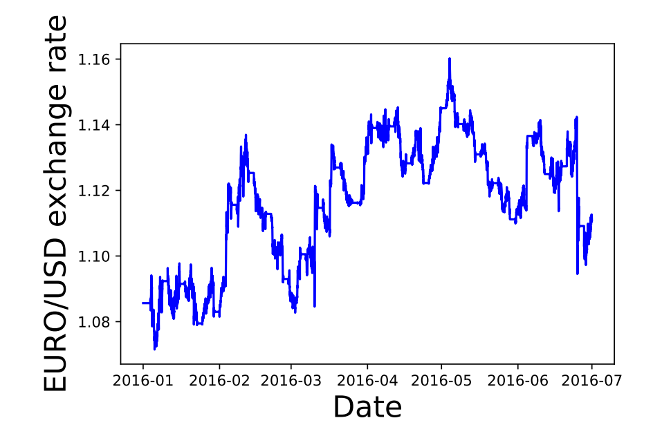
One important type of financial time series is the exchange rate between different currencies (Fig. 1). An exchange rate, is the rate at which one currency will be exchanged for another. There are many factors that can influence this rate, such as balance of payments, interest rate levels, inflation levels and other economical factors which are beyond the scope of this project [3].

Project Statement

The main objective of this project will be to use classical and more recent machine learning techiques to make forecasts of different time series with the goal of applying the best methods to predict currency exchange rates. The simplest model that we will use is the ARIMA model, defined in the previous section as the baseline model. The ARIMA model has been shown to be adequate in estimating the exchange rates of certain currencies Ref. [2]. We will then use different neural networks architectures such as the feed forward and long-short term memory networks, as in Ref. [5; 4; 6], to make predictions of time series and use our baseline models and root mean square differences to quantify and compare the performance of different forecasts.

Metrics

There are several metrics that can be used to evaluate the predictions of our models Ref. [1], however, for our project we will focus on three commonly used metrics, the mean squared error, root mean squared error, and the Akaike information criterion. First we define some terminology, the forecast error, \(e_t\), is \(e_{t} = X_t - F_t,\) where \(X_t\) is the value of the time series at time step \(t\) and \(F_t\) is the forecasted value at the same time step. The three metrics that we will use for our project are

1. The mean square error (MSE)

   • \[\text{MSE} = \frac{1}{N}\sum\limits_{t=1}^{N} e^2_{t}\]

2. The root mean squared error (RMSE)

   • \[\text{RMSE} = \sqrt{\frac{1}{N}\sum\limits_{t=1}^{N} e^2_{t}}\]

3. The Akaike information criterion (AIC)

   • \[\text{AIC} = 2k - \text{Ln}(\hat{L})\]

   where \(k\) is the number of parameters in the model and \(\hat{L}\) is the maximum value of the likelyhood function for the model.

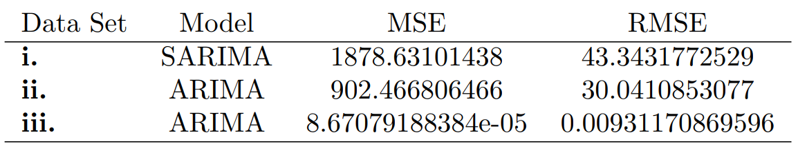
The MSE and RMSE metrics were chosen because, unlike other metrics such as the mean-absolute error (MAE), the MSE and RMSE more strongly penalize the forecast error \(e_t\) due to their quadratic dependence \(e^2_t\). Therefore, large deviations of the forecast to the true data are strongly penalized. Because I was interested in forecasting models which strongly penalized outliers in the forecasts, the MSE and RMSE metrics were the most appropriate. The AIC metric was chosen for evaluating the ARIMA and SARIMA models because it is a well established method for ARIMA and SARIMA models. The AIC scores the specified model on the assumption that the true model of the underlying time series is of higher dimensions than what is being evaluated. Another metric that would be appropriate is the Bayesian information criterion (BIC). The Bayesian information criterion will penalize models more based on the number of present parameters. However, since the AIC has been shown to be asymptotically equivilent to cross-validation [11], it will produce better fits than the BIC metric and was the reason that we chose it. In these three cases, the smaller that the value of the RMSE, MSE, and AIC is, then the better the overall model.

Analysis

Data Exploration

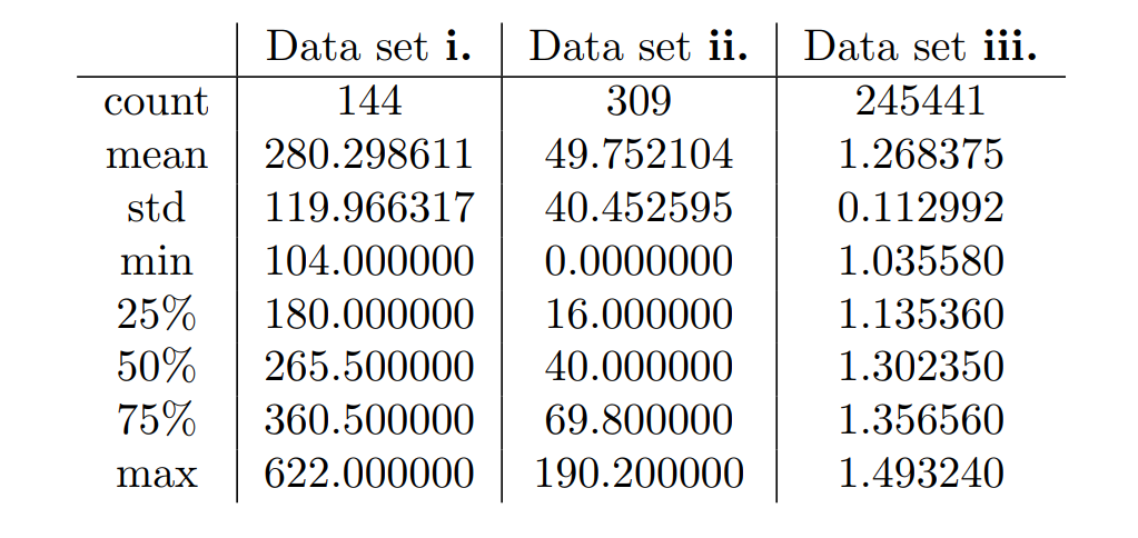
We focused on three time series data sets.

• i. The international airline passenger data set, containing the total number of airline passengers in thousands from Jan 1949 until Dec 1960;

• ii. The sunspot data set, showing the monthly number of sunspots from 1705-1989;

• iii. The EUR to USD exchange rate from Jan 2016- July 2016.

Datasets i. and ii.  both consist of two columns, one for the time steps \(t\) and the values being measured \(X_t\).

The third data set, iii. contains several columns related to the exchange rate market. The columns are Time, the Opening rate, the maximum value of the rate , the lowest value , the closing exchange rate value, and the total volume of the exchange market.

To help us better understand our datasets, in Table 3, we give the computed descriptive statistics of our three data sets in comparison to one-another.

Exploratory Visualization

To understand the data in a more visual way, in the figures below, we plot the times series data sets that we will be analyzing.

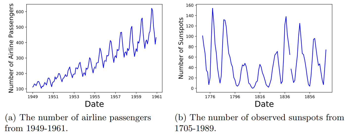
The airline data set in Fig. 2a shows two interesting patterns, the general increasing number of airline passengers over time, along with a seasonal yearly pattern. The sunspot data set in Fig. 2b shows a cyclical pattern that repeats about every 11-years.

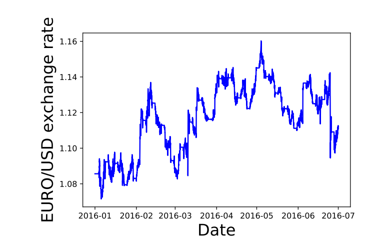
In Fig. 3 we plot the Euro to USD closing price from Jan 2016 to July 2016. There does not seem to be any apparent seasonal or cyclical patterns in this data sample.

Algorithms and Techniques

For this project, we will use the ARIMA model as a benchmark model as described in Sec. Overview and implemented as in Sec. Neural Network Model. ARIMA models have been used to predict foreign exchange rates [2] and are a classical method for time series forecasts Ref. [1]. For these reasons, we use the ARIMA model as a benchmark.

Neural networks for time series models have been explored in the literature [1; 4; 5] and have shown good predictive abilities. This motivates us to explore neural networks for our forecasts. The two neural networks that we will use is the feed-forward neural network with a variable number of nodes along with a long-short-term memory network with a variable number of LSTM units. These networks are shown schematically in Figs. 4 and 5 in the case of 4 nodes and 4 LSTM units. The tutorials in Refs. [7; 6; 8] were very instructive in getting started with these models.

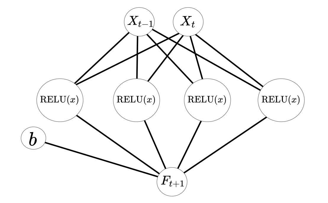
In this diagram, \({X_{t-1},X_{t}}\) is the time series pair that is fed into the neural network, \({\rm RELU}(x)\) is the rectified linear unit activation function of the network, \(b\) is the bias parameter, and \(F_{t}\) is the forecast of the model.

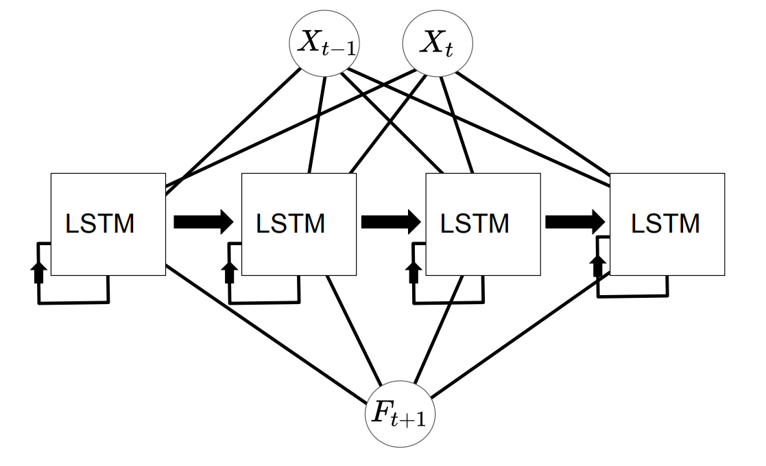
As in the previous diagram, \({X_{t-1},X_{t}}\) is the time series pair. The LSTM blocks represent the long-short-term memory units which feed out-put data back into themselves and \(F_{t}\) is the prediction. In both of the cases, the final model is able to generate a prediction \(F_{t+1}\) for the time series based on the value of the time series at the current time step \(X_{t}\). In Sec. Neural Network Model, we will discus how these architectures were implemented in python.

Benchmark

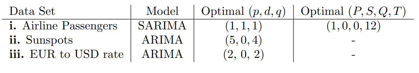
The ARIMA model and seasonal ARIMA model were fit with optimized grid-search parameters, as described in Sec. Neural Network Model, with optimized parameters given in Table 5. In Fig. 6a, Fig. 6b and Fig. 7 the curve in blue is the training data used for fitting, the green line in the testing data and the red lines and red shaded area show the average value of the ARIMA forecast with the 95% confidence regions of the predictions.

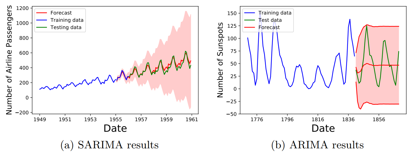
In Fig. 6a, we see that the SARIMA model was able to correctly find the overall trend and as time increases, the forecast uncertainty also increases as would be expected. Fig. 6b which used a ARIMA model, did not seem to to detect the correct trend and produces an uncertainty band that does not change over time. However, the height of the band does overlap with the training data.

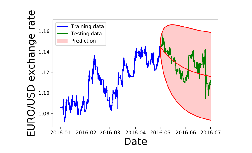
In Fig. 7 above, we see that the ARIMA model did not do a very good job at reproducing the data and it predicts a decreasing trend over time. The uncertainty band is very large in this case and encompasses a wide scale. In Table [table: RMS values of benchmark models], we provide the MSE and RMSE values of the optimized ARIMA and SARIMA models for the above data sets.

Methodology

Data Preprocessing

The forecasting models that we used in this work only require the values \((t,X_t)\), since the data sets that we used do not contain any missing values, our data sets did not require any cleanup. However, it was necessary to scale the data, from \(X_t \rightarrow \tilde{X}_t\) for the neural network data so that it was in the range \([0,1]\). This transformation was accomplished using the following scaling function

where \(X_{\rm max}, X_{\rm min}\) are the maximal and minimum values of the data sets, respectively. This is implemented in python as the following code snippet.

1
2
3
4
5
6
7
8
9
10
11
    def scale_array(y_vec):
        
        ymax = np.max(y_vec)
        ymin = np.min(y_vec)
        
        y_vec_scaled = np.zeros((len(y_vec),1))
        
        for k in range(0,len(y_vec)):
            y_vec_scaled[k][0] = (y_vec[k][0]-ymin)/(ymax-ymin)
        
        return y_vec_scaled,ymin,ymax

To invert the value from the scaling function, we use,

The inversion of the transformation was carried out after the model made its predictions so that the predictions would be in the original range of the data set. This is implemented as follows,

1
2
3
4
5
6
7
    def invert_scaling(y_vec_scaled,ymin,ymax):
        
        y_vec = np.zeros(y_vec_scaled.shape)
            
        for k in range(0,len(y_vec_scaled)):
            y_vec[k] = ymin+(ymax-ymin)*y_vec_scaled[k]
        return y_vec

In order to train the neural network models, we used the following arrays as our feature matrix $X$ and the training data \(y\)

In order to generate these two arrays we used the following function

1
2
3
4
5
6
7
8
9
10
11
12
13
    def future_data(data,lags=1,future=1):
        '''
        This function, takes in the time series [X_t] and returns the array
        X=[X_{t}]
        Y=[X_{t+1}]
        '''
        
        X, y = [], []
        for row in range(len(data) - lags - future):
            a = data[row:(row + lags), 0]
            X.append(a)
            y.append(data[row + lags+future-1, 0])
        return np.array(X), np.array(y)

Another data prepossessing step that we carried out was to separate out the data into training vs testing data sets. The usual amount of training vs testing was about 60-80% for training and 30-40% testing.

There were some additional complications that arose during the coding phases. These complications were related to the some formatting issues that I was not used to.

• The statsmodel package expected the dataframe containing the pandas data frame to have a specific time-format. It took me some time to learn that when I read in data into the dataframe, I needed to use the dataframe.strftime("%Y-%m") to set the column correctly.

• It was difficult to find the correct batch size number for fitting the model, when I used a large number, the resulting models seemed to do very poorly which was counter-intuitive. Smaller batch sizes seemed to give better results.

• The more parameters I was optimizing with the grid search, the longer the runtime. This was a problem with the LSTM network where it was particularly slow.

ARIMA Model: Implementation

We used the ARIMA and the Seasonal ARIMA models from the python package statsmodels (Ref. [10]). The ARIMA model consists of the variables \((p,d,q)\), which are the non-seasonal AR order, differencing, and MA order, respectively. In order to fit this model to data, we use grid search from \((p,d,q)=(0,0,0) \rightarrow (p_{\rm Max},d_{\rm Max},q_{\rm Max})\). To fit the ARIMA model we chose to either minimize the AIC, or the root mean square (RMS) value. The following code generates the grid that we will use to search the model space for the best fitting ARIMA model,

1
2
3
4
5
6
        p = range(0,pMax+1)
        d = range(0,dMax+1)
        q = range(0,qMax+1)
        
        # This creates all combinations of p,q,d
        pdq = list(itertools.product(p, d, q))

For each item in the grid generated with the previous code snippet, we fit ARIMA\((p,d,q)\) model using the following code.

1
2
    for param in pdq:
            arma_mod = statsmodels.tsa.arima_model.ARIMA(train_data,order=param).fit()

Once the model is fit, the AIC or RMS value is computed and the set of parameters \((p,d,q)\) that generated the best score is taken to be the optimal model.

The seasonal ARIMA model incorporates non-seasonal and seasonal factors as a multiplicative model. Therefore, we can schematically write

where the variables \((p,d,q)\) are the non-seasonal AR order, differencing, and MA order, respectively. The variables \((P,D,Q)\) denote the same variables, except for the seasonal component \(S\). The variable \(T\) denotes the number of time steps for a single period. For example, if the time units are in months, then \(T\)=6 indicates a half-year seasonal pattern. In order to fit the SARIMA\((p,q,d,P,D,Q,T)\) model to data, we use a gridsearch. The following code snippet generates a grid of \((p,d,q)=(0,0,0) \rightarrow (p_{\rm Max},d_{\rm Max},q_{\rm Max})\) and \((P,D,Q)=(0,0,0) \rightarrow (p_{\rm Max},d_{\rm Max},q_{\rm Max},T)\), where we take \(T\) as fixed, for simplicity.

1
2
3
4
5
6
7
8
9
10
        p = range(0,pMax+1)
        d = range(0,dMax+1)
        q = range(0,qMax+1)
        t = [t]
        
        # This creates all combinations of p,q,d
        pdq = list(itertools.product(p, d, q))
        
        # This creates all combinations of the seasonal variables
        seasonal_pdq = [(x[0], x[1], x[2], x[3]) for x in list(itertools.product(p, d, q,t))]

For each combination, \((p,q,d,P,D,Q,T)\), we fit the SARIMA model using the code below.

1
2
3
4
5
6
7
8
        for param in pdq:
            for param_seasonal in seasonal_pdq:
                        mod = sm.tsa.statespace.SARIMAX(train_data,
                                                        order=param,
                                      seasonal_order=param_seasonal,
                                         enforce_stationarity=False,
                                        enforce_invertibility=False)
                       results = mod.fit()

Using the above prescription for fitting the ARIMA and SARIMA models, the following table summarizes the results of the gridsearch.

Neural Network Model: Implementation

The feed-forward neural network in Fig. 4 is implemented in Keras. In order to find the optimal number of nodes in this model, we performed a cross-validated grid-search of the parameters neurons (the number of nodes to use in the network) and the batch_size (the number of training samples used in one iteration during training). The cross validation was performed using the following code snippet, which constructs the model in the function build_model(neurons) and then finds the best fit using the GridSearchCV function.

1
2
3
4
5
6
7
8
9
10
11
12
13
14
15
16
17
18
19
20
21
22
23
24
25
26
27
28
    from sklearn.model_selection import GridSearchCV
    from keras.wrappers.scikit_learn import KerasRegressor

    def build_model(neurons):
       '''
       This function build the Feed Forward Neural Network model with a variable number of nodes.
       '''
        model = Sequential()
        model.add(Dense(neurons, input_dim=lags, activation=activation_func))
        model.add(Dense(1))
        model.compile(loss='mean_squared_error', optimizer='adam')
        return model

    # Construct the Regressor model
    regressor = KerasRegressor(build_fn = build_model,verbose=0)
    parameters = {'batch_size': [5,10,20], # Take half of the training data
                  'epochs': [number_of_epochs],
                  'neurons': [4,5,10,15,20]}
                  
    grid_search = GridSearchCV(estimator = regressor,
                               param_grid = parameters,
                               scoring = 'neg_mean_squared_error',
                               cv = 10)
                               
    # Fit the various models using the object defined above
    grid_search = grid_search.fit(X_train, y_train)
    best_parameters = grid_search.best_params_
    best_accuracy = grid_search.best_score_

Once the optimal parameters have been found, we construct this model with the following code snippet that also using the mean_squared_error metric and the adam optimizer.

1
2
3
4
5
    # Now we build and train the optimal model
    model = build_model(neurons=best_parameters['neurons'])

    # Store the history of loss of the optimal function
    history=model.fit(X_train, y_train, epochs=best_parameters['epochs'], batch_size=best_parameters['batch_size'], verbose=0)

The following is an example summary of this implemented architecture (when the optimal nodes is four)

1
2
3
4
5
6
7
8
9
10
    Layer (type)                 Output Shape              Param #   
    =================================================================
    dense_1 (Dense)              (None, 4)                 8         
    _________________________________________________________________
    dense_2 (Dense)              (None, 1)                 5         
    =================================================================
    Total params: 13
    Trainable params: 13
    Non-trainable params: 0
    _________________________________________________________________

Using the same optimizer, loss function and the GridSearchCV object as the feed-forward neural network the LSTM network is implemented as follows

1
2
3
4
5
6
    def build_model(neurons):
        model = Sequential()
        model.add(Dense(neurons, input_dim=lags, activation=activation_func))
        model.add(Dense(1))
        model.compile(loss='mean_squared_error', optimizer='adam')
        return model

Below, we give and example of the LSTM network summary of an implemented LSTM network in the case that the optimal model had four LSTM units,

1
2
3
4
5
6
7
8
9
10
    Layer (type)                 Output Shape              Param #   
    =================================================================
    lstm_1 (LSTM)                (None, 4)                 96        
    _________________________________________________________________
    dense_1 (Dense)              (None, 1)                 5         
    =================================================================
    Total params: 101
    Trainable params: 101
    Non-trainable params: 0
    _________________________________________________________________

Results

Model Evaluation and Validation

Having implemented the feed forward and LSTM networks in Keras as described in Sec. Neural Network Model we fit the model and generate the time series predictions \(\lbrace F_t \rbrace\). One issue that we had using this model was that the predictions of the neural networks do not produce any uncertainties. To try to probe the uncertainties of the model, we carried out the following procedure

1. Train the model using the set \(\lbrace X_{T,{\rm Train}} \rbrace\)

2. Using the training data, calculate the predictions \(\lbrace F_{T,{\rm Train}} \rbrace\)

3. Compute the mean squared error (RMSE), and the standard deviation $\sigma_{\rm RMS}$ between the training set \(X_{T,{\rm Train}}\) and the prediction on the training set \(F_T\).

4. We generate the perturbation, \(\delta X_{T}\), assumed to be a Gaussian random variable sampled from the distribution \(\mathcal{N}(\frac{1}{2}{\rm RMS},\frac{1}{2}\sigma_{\rm RMS} )\)

5. We added the perturbation to the test data \(X_T +\delta X_{T}\) and generate predictions on the testing set, \(\lbrace F_{T,{\rm Test}} \rbrace\).

6. We repeat this process many times, until we generate a distribution of forecasts. The distribution of the forecasts will be the estimated uncertainty of the neural network predictions.

Using this procedure, we generated the uncertainty bands in Figs. 8,9,10.

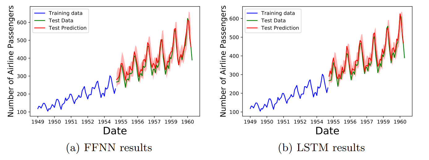
In Fig. 8 we plot the predictions of the feed forward and LSTM neural networks for the Airline passengers dataset. In both cases the red uncertainty band overlap the actual training data, indicating a good fit.

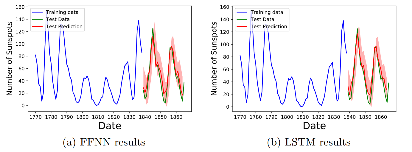
In Fig. 9 we show the comparison of the FFNN and LSTM results for the sunspot dataset. In this case we also see that the uncertainty bands are in agreement with the training data.

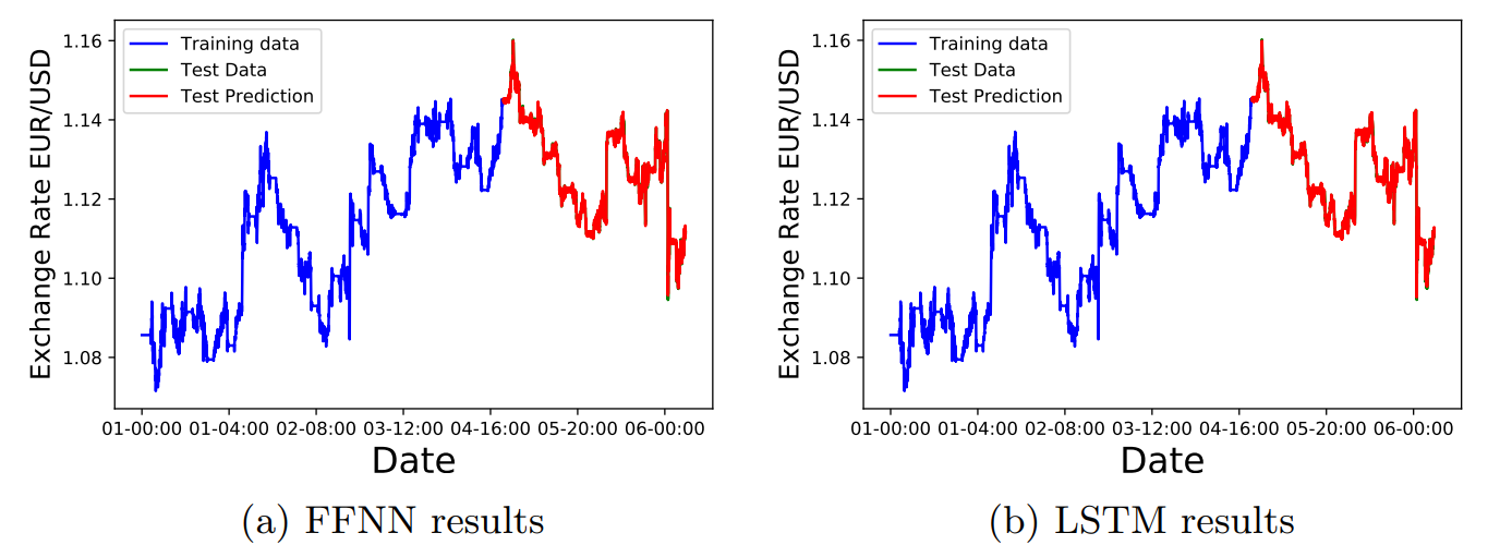
In Fig. 10 we show the results of the FFNN and LSTM networks on the Euro to USD exchange rate. In this case the estimated uncertainty was very small, therefore the uncertainty bands are not visible in the scale of the figure.

Justification

In Table 6, we give the final MSE and RMSE values of all models considered in this project. The RMSE baseline ratio is the value of the RMSE of the baseline model over the RMSE value of the specific model. The larger this ratio, the better the selected model is compared to the baseline model.

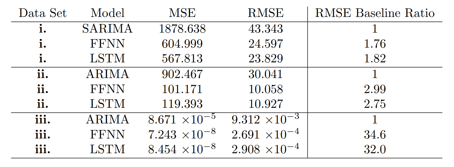
In all three cases, we have that the FFNN and LSTM models outperformed the baseline SARIMA and ARIMA models¹. The FFNN and LSTM models for data sets i. outperformed the baseline by a factor of 1.8, while in data set ii. they outperformed the baseline roughly by a factor of 3. For dataset iii., the FFNN and LSTM models outperformed the baseline by a factor of about 30. We also observed that in some data sets, the LSTM models outperformed the FFNN models by a small margin, however as a rigorous statistical analysis of the RMS and RMSE metrics were not carried out in this project, this small difference is probably not statistically significant.

Conclusion

Limitations

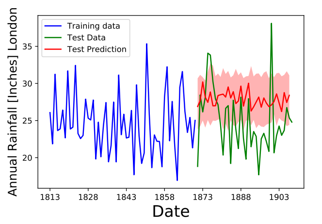
While we had a good amount of success in making models for the time series we considered, it is important to note that not all time series can be tackled using the neural network architectures in this project. There were cases where good fits did not seem to be possible, like the “Annual rainfall in London (in inches)” data set shown in the figure below. When I first looked at this data set, I tried to fit it using the methods that I described in this project, but I obtained very poor results, as pictured in Fig. 11. I tried increasing the training set, changing the activation functions, adding more nodes, but it did not fix the quality of the prediction. It would be very interesting in the future to investigate why this type of time series did not produce good results.

Reflection

In this project we have taken data for time series data \((t,X_t)\) and we have trained two different neural network models, the feed forward neural network (FFNN) and the Long-short term memory (LSTM) network, denoted as \(G_{\rm FFNN}\) ,\(G_{\rm LSTM}\) respectively; to generate a time series forecast given the value of the time series at the previous time step. In other words, we have generated a function \(G\) such that

where \(F_{t+1}\) should be similar to the \(X_{t+1}\) value of the underlying time series data. This problem was very interesting to me as it introduced me to how complicated and difficult time-series analysis can be, the body of literature that studies this subject is large, so it was great to be able to learn a little about it. The project had some challenges, mainly in getting started and in trying to understand the different approaches to time series modeling. The final model worked better than I expected and it is worth investigating in a more rigorous fashion. The fact that the FFNN and LSTM models outperformed the baseline by such a large margin for the EUR/USD exchange rate data suggests that perhaps the model was over-fitting. In the future, I would like to carry out more stringent tests to check against the over-fitting hypothesis.

Improvements

There are some further improvements that we could have carried out to the implemented models, such as an in-depth exploration of different neural network topologies. Adding more adding more layers would have been interesting to explore. However I ran out of time before I could carry out such a careful study. In the future I would also like to implement a generative adversarial artificial neural network for time series prediction. There was not enough time to understand and implement this model, but it seemed quite interesting and powerful. I will try to extend my project in the future to do this.

References

[1]. R. Adhikari and R. K. Agrawal, An Introductory Study on Time Series Modeling and Forecasting, 2013, [arXiv:1302.6613]

[2]. T. Mong and U. Ngan, Research Journal of Finance and Accounting www.iiste.org ISSN 2222-1697 (Paper) ISSN 2222-2847 (Online) Vol.7, No.12, 2016.

[3] P. J. Patel, N. J. Patel and A. R. Patel, IJAIEM 3, 3, 2014.

[4] B. Oancea, S. Cristian Ciucu, Proceedings of the CKS 2013, [arXiv:1401.1333].

[5] T. D. Chaudhuri and I. Ghosh, Journal of Insurance and Financial Management, Vol. 1, Issue 5, PP. 92-123, 2016, [arXiv:1607.02093].

[6] Pant, N. (2017, September 07). A Guide For Time Series Prediction Using Recurrent Neural Networks (LSTMs).

[7] D. K. Acatay, (2017, Nov. 21) Part 6: Time Series Prediction with Neural Networks in Python.

[8] Vincent, T. (2018). ARIMA Time Series Data Forecasting and Visualization in Python | DigitalOcean. [online] digitalocean.com. [Accessed 29 Jul. 2018].

[9] C. Esteban, S. L. Hyland and G Rätsch, [arXiv:1706.02633].

[10] S. Skipper and J. Perktold. “Statsmodels: Econometric and statistical modeling with python.” Proceedings of the 9th Python in Science Conference. 2010.

[11] Stone, M. “An Asymptotic Equivalence of Choice of Model by Cross-Validation and Akaike’s Criterion.” Journal of the Royal Statistical Society. Series B (Methodological), vol. 39, no. 1, 1977, pp. 44–47. JSTOR, JSTOR,