Precision, Recall and all that
Let us now consider a binary classification task. Our training data is denoted as the set \({\bf T}\), where
\[{\bf T} = \lbrace (x_i,y_i)| i=1,...,N \rbrace\]Our data vector \({\bf y}\) can have two outcomes, \(y_k= 0 \text{ or } 1\). Let us call the outcome with a +1 value, be the positive value while the 0 is called the negative value.
Table of Contents
- Accuracy
- Precision
- Recall
- The F Metric
- The ROC curve
- The link between accuracy, recall and precision
Definitions
For our binary classifier model trained on \(T\) is denoted as \(\hat{g}_T.\) The number of positive samples in \(T\) is \(N_p\), while the number of negative samples is \(N_n\). The total number of samples is $N$,
\[\begin{align} N &= N_p+N_n \\ T_p &= \text{ True Positives} \\ T_n &= \text{ True Negatives} \\ F_p &= \text{ False Positives} \\ F_n &= \text{ False Negatives} \\ N_p &= T_p+F_n \\ N_n &= T_n+F_p \\ N &= T_p+T_n+F_p+F_n. \end{align}\]Furthermore, we denote the estimates of \(N_p\) and \(N_n\) given by our classifier as \(\hat{N}_p\) and \(\hat{N}_n\), \(\hat{N}_p = \text{ Number of positive predictions by classifier}, \\ \hat{N}_n = \text{ Number of negative predictions by classifier}, \\ \hat{N}_p+\hat{N}_n = N.\)
With these definitions we have that the confusion matrix is defined as
\[C= \begin{bmatrix} T_p & F_p\\ F_n & T_n \end{bmatrix}\]when we divide \(C\) by the number of samples, then we can give the confusion matrix a probabilistic interpretation
\[\mathcal{C}= \begin{bmatrix} P({\bf \hat{y}}={\bf 1}|{\bf y}={\bf 1},\hat{g}_T) & P({\bf \hat{y}}={\bf 1}|{\bf y}={\bf 0},\hat{g}_T)\\ P({\bf \hat{y}}={\bf 0}|{\bf y}={\bf 1},\hat{g}_T) & P({\bf \hat{y}}={\bf 0}|{\bf y}={\bf 0},\hat{g}_T) \end{bmatrix}\]In the special case that our classifier doesn’t make any mistakes, the false negatives and positives are zero, therefore
\[C_{\text{Perfect}}= \begin{bmatrix} T_p & 0\\ 0 & T_n \end{bmatrix}\]In the other extreme where the classifier doesn’t make any correct classifications we have
\[\mathcal{C}_{\text{Terrible}}= \begin{bmatrix} 0 & F_p\\ F_n & 0 \end{bmatrix}\]And in the case where the classifier is totally random,
\[\mathcal{C}_{\text{Random}}= \begin{bmatrix} \frac{1}{4} & \frac{1}{4}\\ \frac{1}{4} & \frac{1}{4} \end{bmatrix}\]Accuracy
How well did the classifier get the correct labels.
\[a = P({\bf y}={\bf \hat{y}},\hat{g}_T) \\ = P({\bf y}={\bf \hat{y}}, {\bf y}=1,\hat{g}_T)+P({\bf y}={\bf \hat{y}}, {\bf y}=0,\hat{g}_T)\\ = \left( \frac{T_p}{N} \right) + \left( \frac{T_n}{N} \right) \\ = \frac{T_p+T_n}{N}\] \[0 \leq a \leq 1\]- a perfect classifier would have \(a=1\).
- a terrible classifier has \(a=0\)
- a random classifier has \(a=\frac{1}{2}\)
Precision
Of the samples, \(\hat{N}_p\), that the classifier thought were positive, how many are actually correct ?
\[p = P({\bf y}={\bf 1}| {\bf \hat{y}} = {\bf 1},\hat{g}_T) \\ = \frac{T_p}{\hat{N}_p} \\ = \frac{T_p}{T_p+F_p}\] \[0 \leq p \leq 1\]- a perfect classifier would have \(p=1\).
- a terrible classifier has \(p=0\)
- a random classifier has \(p=\frac{1}{2}\)
Recall
Recall, is the metric that measures the fraction of positively identified samples,
\[r = P( {\bf \hat{y}}={\bf 1} | {\bf y}={\bf 1},\hat{g}_T) \\ = \frac{T_p}{N_p} \\ = \frac{T_p}{T_p+F_n}\] \[0 \leq r \leq 1\]- a perfect classifier would have \(r=1\).
- a terrible classifier has \(r=0\)
- a random classifier has \(r=\frac{1}{2}\)
The F Metric
The \(F_\beta\) metric is the following function of precision and recall.
\[F_{\beta} = (1+\beta^2) \frac{p r}{\beta^2p+r}\]clearly
\[0 \leq F_\beta \leq 1\]In the case where \(\beta\)=1, then \(F_1\) is the harmonic mean of the precision and recall
\[F_1 = \frac{2pr}{r+p}\]- a perfect classifier would have \(F_\beta=1\),
- a terrible classifier has \(F_\beta=0\),
- a random classifier has \(F_\beta=\frac{1}{2}\).
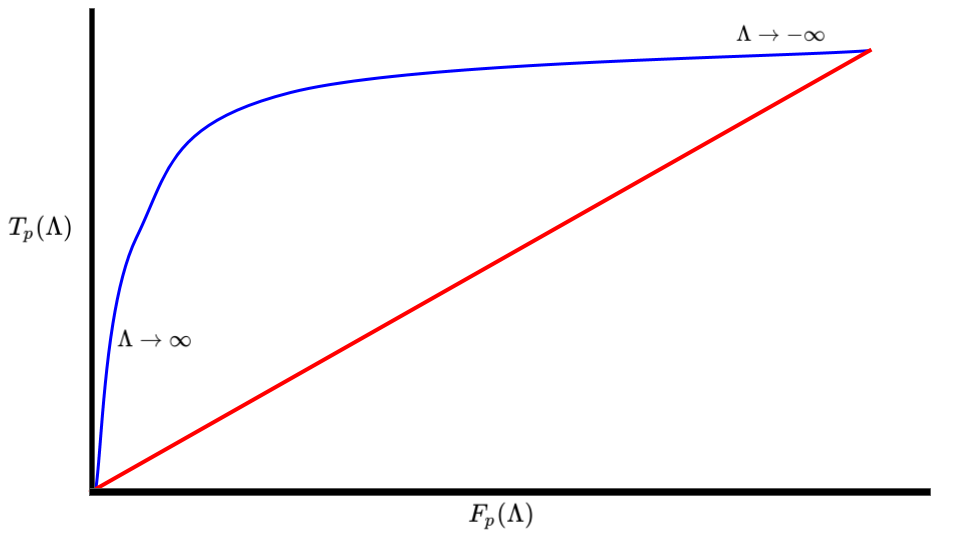
ROC curve
The Receiver operator curve is the plot generated when one plots the True positive rate \(T_p\) vs the False positive rate \(F_p\) for a classifier that depends on a parameter \(\Lambda\).
The area \(\mathcal{A}\) of the ROC curve can be interpreted as the probability that a random sample \(x\) such that \(x \in P\) will be classified as a True positive, compared to a False Positive. The area also satisfies the following properties,
- a perfect classifier would have \(\mathcal{A}=1\),
- a terrible classifier has \(\mathcal{A}=0\),
- a random classifier has \(\mathcal{A}=\frac{1}{2}\).
Mathematical Details
Let us suppose that we have a classifier \(g\) such that,
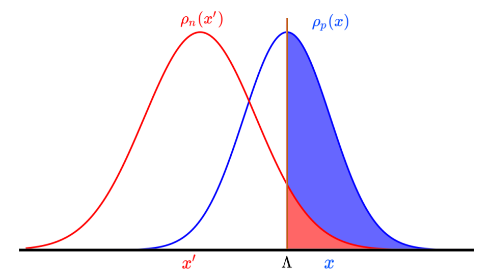
\[g(x,\Lambda) = \Bigg\{ \begin{matrix} 1 \quad \text{ if } x \geq \Lambda \\ 0 \quad \text{ if } x < \Lambda \end{matrix}\]for a given \(x\) and \(\Lambda\). In addition, there exists distributions \(\rho_p(x)\) and \(\rho_n(x)\) that represent the true positive distribution and true negative distributions, respectively, that we are trying to distinguish with our classifier \(g(x,\Lambda)\). With this classifier, we have the following values for the confusion matrix \(C\),
\[T_p(\Lambda) = N_p \int\limits_{\Lambda}^{\infty} dx \ \rho_p(x), \\ F_p(\Lambda) = N_n \int\limits_{\Lambda}^{\infty} dx \ \rho_n(x), \\ T_n(\Lambda) = N_n \int\limits_{-\infty}^{\Lambda} dx \ \rho_n(x), \\ F_n(\Lambda) = N_p \int\limits_{-\infty}^{\Lambda} dx \ \rho_p(x).\]In Fig 2, the solid blue area represents the \(T_p(\Lambda)\) value, while the red area is the \(F_p(\Lambda)\) values.
With these definitions, let us now compute the area of the ROC, \(\mathcal{A}\). Note that since as \(\Lambda \rightarrow \infty\), then \(T_p \rightarrow 0\), and so we compute the area with the limits ranging from \(\infty < dF_p < -\infty\),
\[\mathcal{A} = \int \limits_{\infty}^{-\infty} \ T_p(\Lambda) dF_p(\Lambda) \\ = -\int \limits_{-\infty}^{\infty} d\Lambda \ T_p(\Lambda) \frac{dF_p}{d\Lambda}(\Lambda) \\ = N_n \int \limits_{-\infty}^{\infty} d\Lambda \ T_p(\Lambda) \rho_n(\Lambda) \\ = N_n N_p \int \limits_{-\infty}^{\infty} d\Lambda \ \rho_n(\Lambda) \int \limits_{\Lambda}^{\infty} dx \ \rho_p(x) \\ = N_n N_p \int \limits_{-\infty}^{\infty} d\Lambda \ \rho_n(\Lambda) \int \limits_{-\infty}^{\infty} dx \ \theta(x-\Lambda)\rho_p(x) \\ = N_n N_p \int \limits_{-\infty}^{\infty} dx' \ \int \limits_{-\infty}^{\infty} dx \ \theta(x-x')\rho_p(x) \rho_n(x') \\ = P( \rho_p(x) > \rho_n(x) |x\in T_p)\]Connection between Accuracy, Recall and Precision
Having written down Recall and precision as conditional probabilities, it is much
\[P({\bf \hat{y}}={\bf 1}) = \frac{\hat{N}_p}{N} = \frac{T_p+F_p}{N} \\ P({\bf \hat{y}}={\bf 0}) = \frac{\hat{N}_n}{N} = \frac{T_n+F_n}{N} \\ \text{ }\\ P({\bf y}={\bf 1}) = \frac{N_p}{N} = \frac{T_p+F_n}{N} \\ P({\bf y}={\bf 0}) = \frac{N_n}{N} = \frac{T_n+F_p}{N}\]By Bayes theorem we have that
\[P({\bf y}={\bf 1}| {\bf \hat{y}} = {\bf 1}) = \frac{P({\bf \hat{y}} = {\bf 1}|{\bf y}={\bf 1})P({\bf y}={\bf 1})}{P({\bf \hat{y}}={\bf 1})} \\ = P({\bf \hat{y}} = {\bf 1}|{\bf y}={\bf 1}) \frac{T_p+F_n}{T_p+F_p} \\ = P({\bf \hat{y}} = {\bf 1}|{\bf y}={\bf 1}) \frac{N_p}{\hat{N}_p}\]In otherwords, we find that
\[p = r \left(\frac{N_p}{\hat{N}_p}\right)\]